Build mode support
Summarize replay into representative joint actions yk(x), using identity support or joint-action quantization.
NeurIPS 2026
MoSDOT

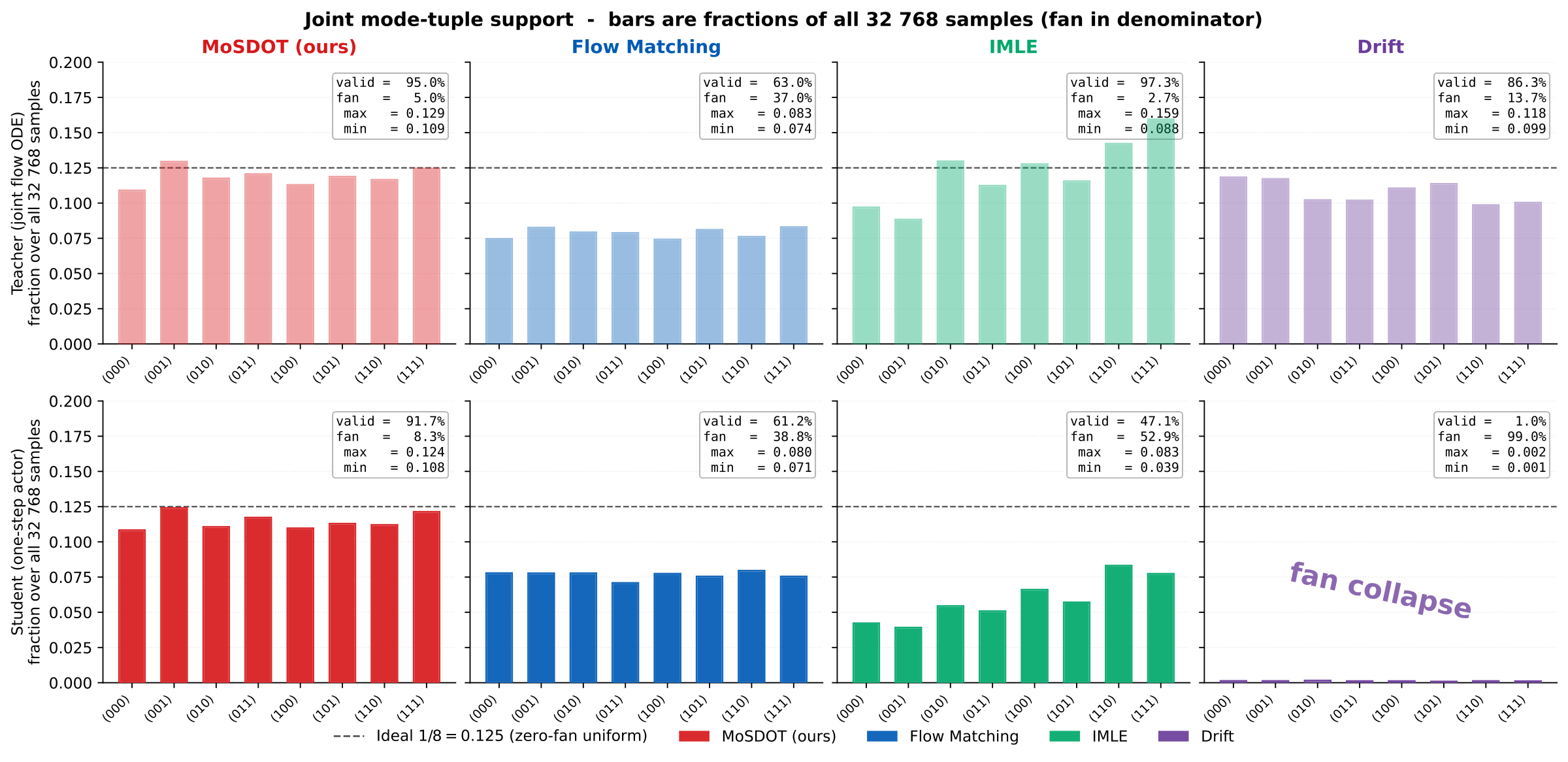
Teacher routing, then distillation. First a 2D toy with trained flow teachers: flow matching pairs noise with targets at random, MoSDOT by SDOT. Then the landmark diagnostic, replaying the paper figure's runs: joint teachers and the one-step students distilled from them. Red marks off-support samples, between valid modes.
TL;DR Better coordination starts with a better teacher: align source noise with joint-action modes, then distill into local one-step policies.
Video
Why multimodal teachers fail under distillation, how source assignment fixes it, and what the agents do on the benchmarks.
Overview. Narration is synthesized (Kokoro TTS); English captions are included. Table values are the paper's; the landmark animation replays the paper figure's runs, and the benchmark footage comes from policies re-trained with the paper configurations.
The problem
Each agent alone has good options. Only some combinations work together, and those combinations are what the teacher must learn and the students must keep.
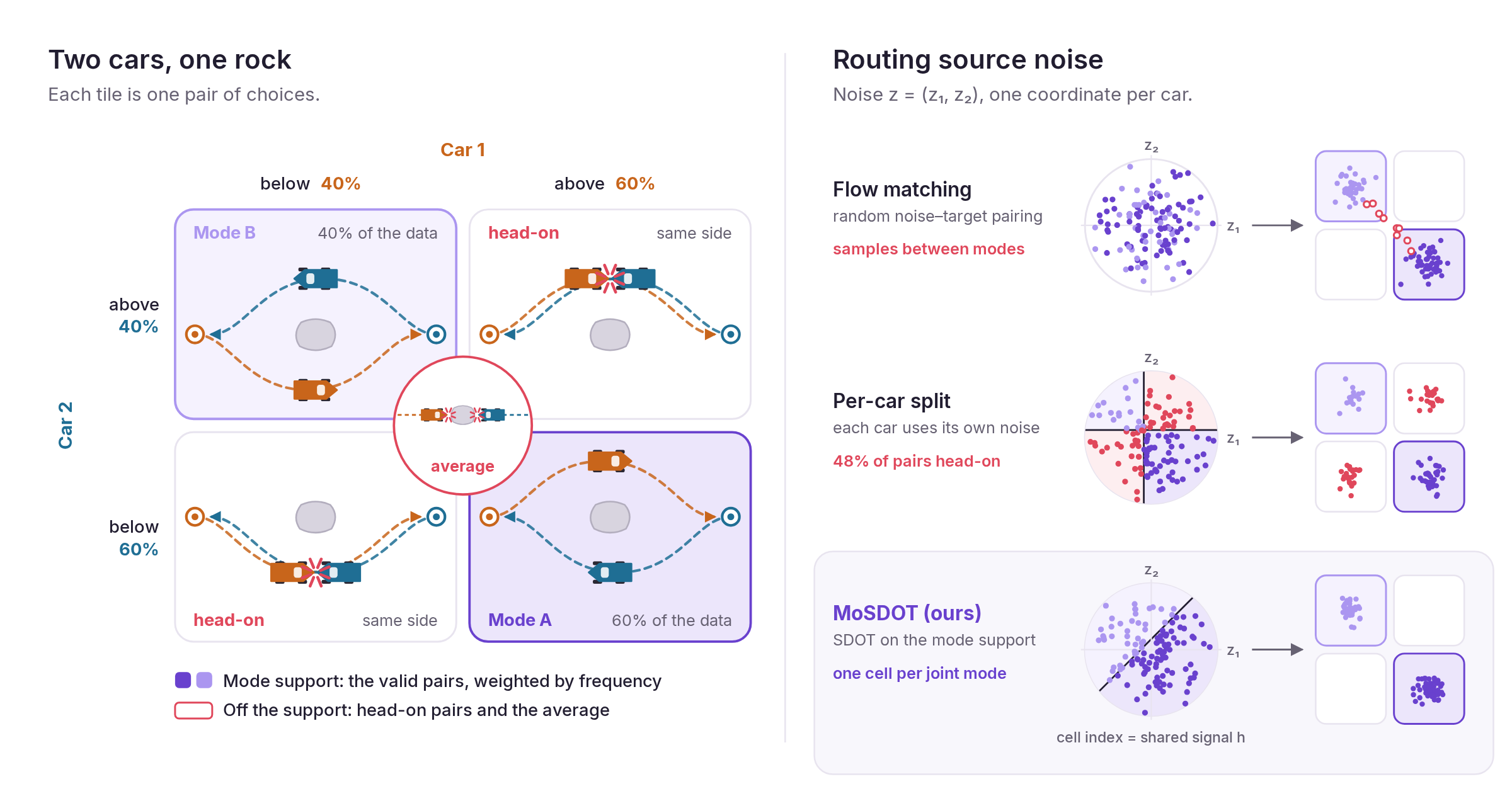
Modes are pairs, not single choices. Either car may pass above or below the rock; only opposite sides get through. Flow matching leaves samples between the two modes, splitting each car's own noise reaches head-on pairs, and MoSDOT gives each joint mode its own noise cell, sized by how often the mode occurs in the data.
The idea
A centralized teacher can reach valid joint-action modes yet still assign nearby noise samples to conflicting behaviors. Local actors can inherit these artifacts during distillation, producing actions between valid modes.
MoSDOT organizes the source-to-mode assignment first. Capacity-matched transport gives the teacher cleaner targets and preserves more of the support that decentralized actors can recover.
A clean teacher does not remove the strict-product gap: independent local policies cannot represent every correlated joint distribution. We study shared randomness separately.
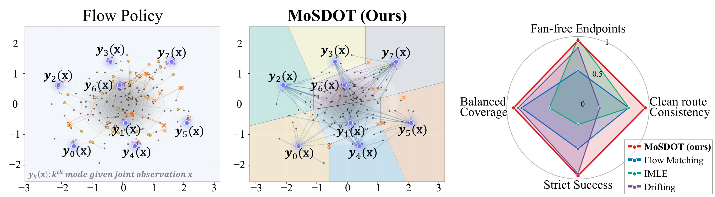
Give every noise sample a coordinated destination. MoSDOT assigns source regions to replay-derived modes before teacher training, reducing off-support mass and improving routing consistency.
Landmark means over 4 seeds (Table 1). Benchmark averages as reported in Tables 2–3; benchmark evaluation uses 6 seeds.
The method
A structured source assignment before teacher training.
One-step local actors at execution.
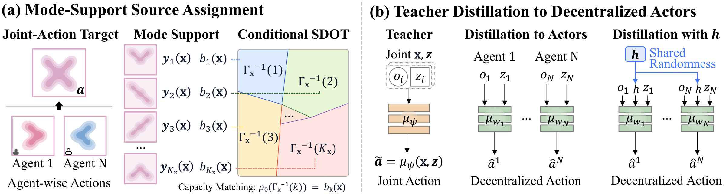
The MoSDOT framework. Transport operates on coordinated joint-action modes. Each distilled actor uses its own observation and noise; the shared-randomness variant additionally supplies a common signal h.
Summarize replay into representative joint actions yk(x), using identity support or joint-action quantization.
Assign each mode a target source mass bk(x) from its empirical replay frequency.
Partition source noise into capacity-matched Laguerre cells, each assigned to one joint-action mode.
Train the teacher on aligned paths and distill its joint actions into decentralized one-step policies.
Benchmark results
Strong gains on diverse continuous replay, with results that vary by discrete-action regime. Explore every baseline and dataset below.
Continuous actions · four dataset qualities
| Method | Expert ↑ | Medium ↑ | Medium-Replay ↑ | Random ↑ | Average ↑ |
|---|---|---|---|---|---|
| MATD3BC | 108.3 ± 3.3 | 29.3 ± 4.8 | 15.4 ± 5.6 | 9.8 ± 4.9 | 40.7 |
| MACQL | 98.2 ± 5.2 | 34.1 ± 7.2 | 20.0 ± 8.4 | 24.0 ± 9.8 | 44.1 |
| ICQ | 114.9 ± 2.6 | 47.9 ± 18.9 | 37.9 ± 12.3 | 34.4 ± 5.3 | 58.8 |
| OMAR | 104.0 ± 3.4 | 29.3 ± 5.5 | 13.6 ± 5.7 | 6.3 ± 3.5 | 38.3 |
| OMIGA | 80.8 ± 13.8 | 30.1 ± 16.9 | 5.4 ± 11.0 | −3.8 ± 12.3 | 28.1 |
| MADiff | 95.0 ± 5.3 | 64.9 ± 7.7 | 30.3 ± 2.5 | 6.9 ± 3.1 | 49.2 |
| MAC-Flow | 101.7 ± 10.9 | 80.1 ± 20.6 | 50.4 ± 33.2 | 31.1 ± 6.8 | 65.8 |
| MoSDOT Ours | 104.40 ± 19.66 | 95.97 ± 12.69 | 54.12 ± 15.29 | 75.92 ± 23.81 | 82.6 |
MoSDOT leads on Medium, Medium-Replay, and Random; ICQ has the highest Expert mean.
Five scenarios, three dataset qualities.
| Method | Average ↑ |
|---|---|
| BC | 12.2 |
| MABCQ | 5.5 |
| MACQL | 13.1 |
| Diffusion BC | 13.0 |
| MADiff | 13.8 |
| DoF | 15.6 |
| Flow BC | 13.4 |
| MAC-Flow | 15.6 |
| MoSDOT Ours | 16.7 |
| Method | Good ↑ | Medium ↑ | Poor ↑ |
|---|---|---|---|
| BC | 16.0 ± 1.0 | 8.2 ± 0.8 | 4.4 ± 0.1 |
| MABCQ | 3.7 ± 1.1 | 4.0 ± 1.0 | 3.4 ± 1.0 |
| MACQL | 19.1 ± 0.1 | 13.7 ± 0.3 | 4.2 ± 0.1 |
| Diffusion BC | 19.5 ± 0.5 | 13.3 ± 0.7 | 4.2 ± 0.2 |
| MADiff | 19.3 ± 0.5 | 16.4 ± 2.6 | 10.3 ± 6.1 |
| DoF | 19.8 ± 0.2 | 18.6 ± 1.2 | 10.9 ± 1.1 |
| Flow BC | 20.0 ± 0.0 | 14.7 ± 1.5 | 4.5 ± 0.1 |
| MAC-Flow | 19.8 ± 0.2 | 18.0 ± 3.2 | 10.6 ± 2.2 |
| MoSDOT Ours | 20.0 ± 0.0 | 18.8 ± 1.5 | 16.4 ± 4.9 |
| Method | Good ↑ | Medium ↑ | Poor ↑ |
|---|---|---|---|
| BC | 16.7 ± 0.4 | 10.7 ± 0.5 | 5.3 ± 0.1 |
| MABCQ | 4.8 ± 0.6 | 5.6 ± 0.6 | 3.6 ± 0.8 |
| MACQL | 18.9 ± 0.9 | 15.5 ± 1.5 | 7.5 ± 1.0 |
| Diffusion BC | 19.4 ± 0.5 | 18.6 ± 0.6 | 4.8 ± 0.2 |
| MADiff | 18.9 ± 1.1 | 16.8 ± 1.6 | 9.8 ± 0.9 |
| DoF | 19.6 ± 0.3 | 18.6 ± 0.8 | 12.0 ± 1.2 |
| Flow BC | 19.5 ± 0.2 | 18.2 ± 0.8 | 4.9 ± 0.1 |
| MAC-Flow | 19.7 ± 0.3 | 19.4 ± 0.6 | 11.5 ± 0.8 |
| MoSDOT Ours | 20.0 ± 0.0 | 20.0 ± 0.0 | 10.8 ± 0.8 |
| Method | Good ↑ | Medium ↑ | Poor ↑ |
|---|---|---|---|
| BC | 18.2 ± 0.4 | 12.3 ± 0.7 | 6.7 ± 0.3 |
| MABCQ | 7.7 ± 0.9 | 7.6 ± 0.7 | 6.6 ± 0.2 |
| MACQL | 17.4 ± 0.3 | 15.6 ± 0.4 | 8.4 ± 0.8 |
| Diffusion BC | 18.0 ± 1.0 | 13.4 ± 1.4 | 6.2 ± 1.2 |
| MADiff | 15.9 ± 1.2 | 15.6 ± 0.3 | 8.5 ± 1.3 |
| DoF | 18.5 ± 0.8 | 18.1 ± 0.9 | 10.0 ± 1.1 |
| Flow BC | 19.5 ± 0.1 | 15.1 ± 2.0 | 6.9 ± 0.8 |
| MAC-Flow | 19.5 ± 0.5 | 17.6 ± 0.6 | 8.5 ± 0.6 |
| MoSDOT Ours | 20.1 ± 0.1 | 18.2 ± 1.0 | 9.4 ± 0.8 |
| Method | Good ↑ | Medium ↑ | Poor ↑ |
|---|---|---|---|
| BC | 15.8 ± 3.6 | 12.4 ± 0.9 | 7.5 ± 0.2 |
| MABCQ | 2.4 ± 0.4 | 3.8 ± 0.5 | 3.3 ± 0.5 |
| MACQL | 16.2 ± 1.6 | 15.1 ± 2.9 | 10.5 ± 3.1 |
| Diffusion BC | 16.8 ± 2.3 | 12.5 ± 2.1 | 8.0 ± 1.0 |
| MADiff | 16.5 ± 2.8 | 15.2 ± 2.6 | 8.9 ± 1.3 |
| DoF | 17.7 ± 1.1 | 16.2 ± 0.9 | 10.8 ± 0.3 |
| Flow BC | 14.7 ± 2.1 | 12.8 ± 0.8 | 7.7 ± 0.8 |
| MAC-Flow | 18.6 ± 3.5 | 15.6 ± 1.3 | 9.8 ± 2.1 |
| MoSDOT Ours | 18.5 ± 1.9 | 17.9 ± 1.2 | 12.3 ± 0.9 |
| Method | Good ↑ | Medium ↑ | Poor ↑ |
|---|---|---|---|
| BC | 17.5 ± 0.4 | 12.5 ± 0.3 | 9.7 ± 0.2 |
| MABCQ | 10.1 ± 0.2 | 9.9 ± 0.2 | 9.0 ± 0.2 |
| MACQL | 12.9 ± 0.2 | 11.6 ± 0.1 | 10.2 ± 0.1 |
| Diffusion BC | 17.8 ± 1.3 | 10.5 ± 1.1 | 10.2 ± 2.3 |
| MADiff | 14.7 ± 2.2 | 12.8 ± 1.2 | 10.8 ± 1.1 |
| DoF | 16.1 ± 0.8 | 13.9 ± 0.9 | 11.5 ± 1.1 |
| Flow BC | 18.0 ± 1.3 | 11.8 ± 2.6 | 10.0 ± 0.3 |
| MAC-Flow | 19.1 ± 0.8 | 14.9 ± 4.1 | 11.4 ± 0.4 |
| MoSDOT Ours | 20.2 ± 0.6 | 16.4 ± 1.0 | 11.4 ± 1.4 |
Reported average reward: MoSDOT 16.7; MAC-Flow and DoF 15.6. Select a scenario to inspect all means and uncertainties.
Discrete actions · replay datasets
| Method | terran_ | zerg_ | terran_ | Average ↑ |
|---|---|---|---|---|
| BC | 7.3 ± 1.0 | 6.8 ± 0.6 | 7.4 ± 0.5 | 7.2 |
| MABCQ | 13.8 ± 4.4 | 10.3 ± 1.2 | 12.7 ± 2.0 | 12.3 |
| MACQL | 11.8 ± 0.9 | 10.3 ± 3.4 | 11.8 ± 2.0 | 11.3 |
| Diffusion BC | 9.3 ± 0.9 | 8.1 ± 1.7 | 5.5 ± 1.5 | 7.6 |
| MADiff | 13.3 ± 1.8 | 10.2 ± 1.1 | 13.8 ± 1.3 | 12.4 |
| DoF | 15.4 ± 1.3 | 12.0 ± 1.1 | 14.6 ± 1.1 | 14.0 |
| Flow BC | 8.3 ± 1.9 | 4.6 ± 0.5 | 5.8 ± 1.7 | 6.2 |
| MAC-Flow | 16.6 ± 4.3 | 9.8 ± 1.5 | 13.0 ± 4.7 | 13.1 |
| MoSDOT Ours | 16.6 ± 4.3 | 9.7 ± 2.8 | 9.4 ± 2.6 | 11.9 |
DoF has the highest reported average (14.0), followed by MAC-Flow (13.1); MoSDOT reports 11.9.
Mean ± 2σ · 6 seeds · higher is better
Bold best mean Underlined second-best mean · ties included
Tables 2–3 in the paper. Average columns reproduce the reported values without recalculation. Download table data Swipe tables horizontally to see all columns.
MoSDOT's decentralized one-step actors on every benchmark. StarCraft II clips are rendered by the game engine itself during evaluation (MoSDOT red, built-in AI blue). The clips show successful episodes of policies re-trained with the paper configurations.
Looking closer
Controlled diagnostics separate teacher routing quality from the limits of independent local execution.
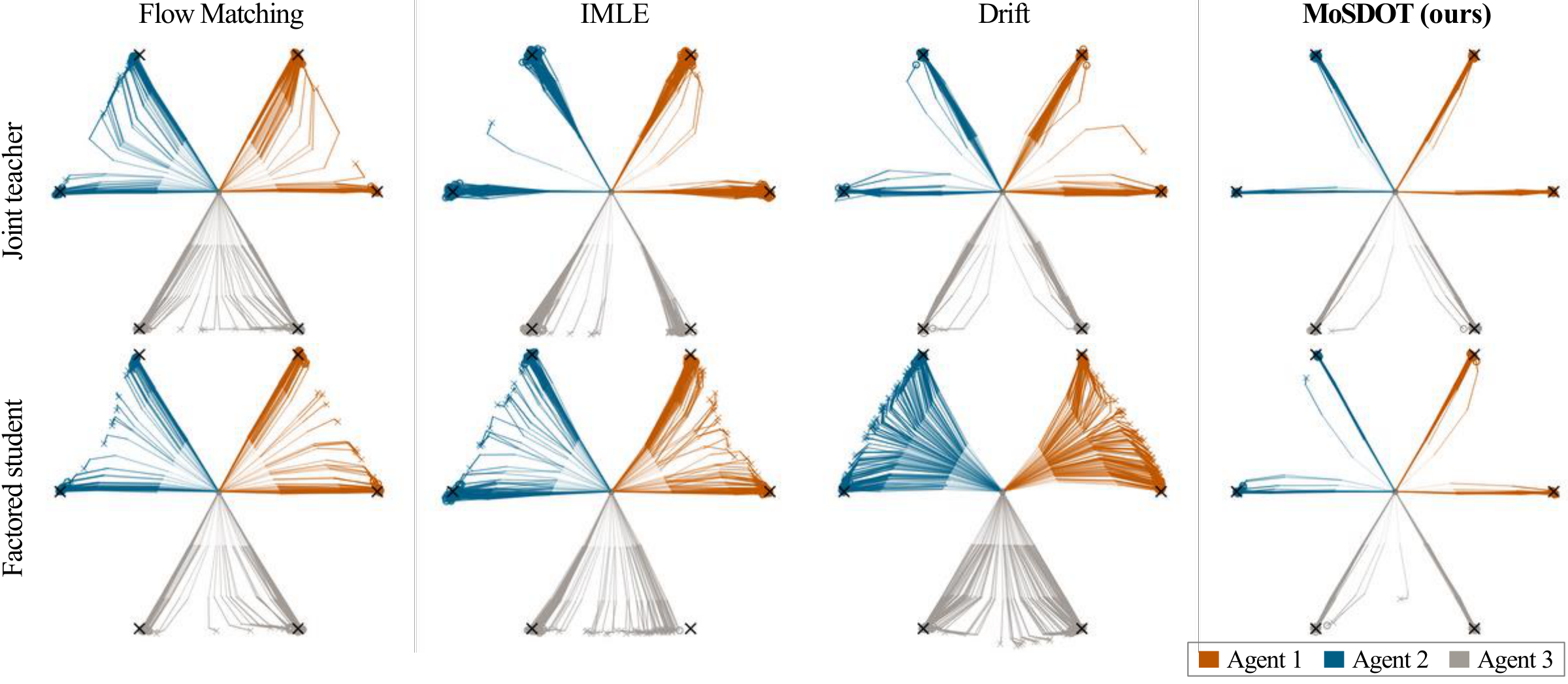
MoSDOT reduces fan mass between modes and retains the teacher’s ray structure after distillation.
Teacher → student. Top: centralized teacher rollouts. Bottom: one-step factorized students with independent local noise. Black crosses mark the six anchor mode endpoints. Animated from the same runs as the paper figure: rollouts are drawn one at a time, and red marks rollouts whose first step leaves both 10° landmark cones (off-support), with a live count per panel.
Joint-teacher landmark diagnostics · Table 1 · mean over 4 seeds
| Method | Fan-free ↑ | Route consistency ↑ | Success ↑ | Balance ↑ |
|---|---|---|---|---|
| Flow matching | 0.857 | 0.856 | 0.915 | 0.917 |
| IMLE | 0.991 | 0.857 | 0.848 | 0.761 |
| Drifting | 0.952 | 0.653 | 0.985 | 0.936 |
| MoSDOT Ours | 0.983 | 0.972 | 0.991 | 0.961 |
IMLE has the highest fan-free score. MoSDOT has the highest route consistency, success, and balance. Bold marks the best mean; underlining marks the second-best.
On XOR, independent local sampling cannot preserve the correlated target support. A shared mode-selection signal lets local actors coordinate.
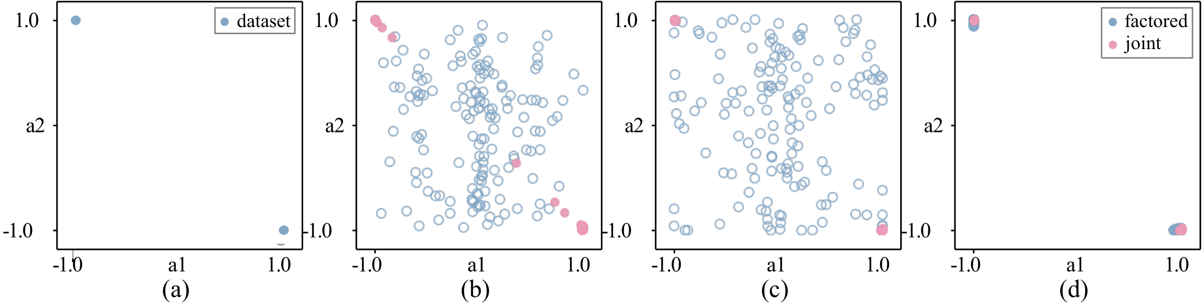
Isolating the strict-product gap. (a) Target support. (b) MAC-Flow. (c) MoSDOT without a shared signal. (d) MoSDOT with a shared signal. Blue: factored student; pink: joint teacher.
Reference
Accepted to NeurIPS 2026.
Sangmin Lee, Youngju Na, Chanmi Lee, and Sung-eui Yoon · KAIST.
@inproceedings{lee2026mosdot,
  title = {Multi-Agent Coordination via
           Support-Preserving Distillation},
  author = {Sangmin Lee and Youngju Na and
            Chanmi Lee and Sung-eui Yoon},
  booktitle = {Advances in Neural Information
               Processing Systems},
  year = {2026}
} ↗ Paper figure